Otometry: Hearing Aid Fitting History

Scientific Prescriptive Fitting Origin

By Wayne J. Staab, PhD

In the late 1950s, a fitting approach called otometry was introduced. It was presented as being based on science rather than on historical practice, supposition, and trial and error, as were the fitting approached used at that time.

Developed by John Victoreen, LLD, otometry was presented as a scientific prescription to hearing aid fitting.^1–5 Victoreen was a self-taught physicist, engineer, inventor, and at the time, the owner of the Vicon Instrument Company, manufacturing hearing aids in Colorado Springs, CO. Otometry is seldom, if ever, used currently, but the approach taken to establish its basic principles have been employed by essentially all current hearing aid fitting formulae, whether recognized or not. As such, this topic has a place in the historical development of the rehabilitative efforts involved in the discipline of hearing. A more detailed account can be found at: http://hearinghealthmatters.org/waynesworld/2014/otometry-least-forget/

Otometry

Otometry was founded on the premise that in order to find the best amplification for a hearing-impaired person, the prosthetic need should be based on normal ear performance. The hearing aid should assist in helping the impaired ear to behave as if it were a normal ear. To this end, the relationships between frequency, sound pressure, and loudness in normal ears were measured, with the goal being to restore these relationships in the impaired ear. And, any amplification prescription should be based on dB SPL, as hearing aid performance was measured, not dB HL as audiograms were recorded. A hearing aid should apply sound pressure to hearing that remains, not to that which is lost. These relationships form the basis for otometry.

Fitting hearing aids, using otometry, was not readily accepted by the audiological and dispensing community. Primary reasons given were: (1) audiology was functioning as a behavioural science (mostly by individuals having social science backgrounds), and as such, it was not comfortable with a fitting procedure that involved physics and acoustics, (2) otometry did not accept the audiogram as part of the hearing aid fitting, but as a tool to measure hearing loss, (3) audiologists were not significantly involved in the fitting of hearing aids, and if remotely involved, suggested fittings based on “mirroring the audiogram,” (4) otometry did not focus on intelligibility because it believed that word recognition scores could not determine or predict the hearing aid properties most useful to a defective ear, and (5) hearing aid dealers had little or no education in physics, hearing disorders, and acoustics – most having come from retail sales.

Basic Principles of Otometry

A reference chart to assist in comparing otometry and audiometry is shown in Figure 1. It shows how various sound pressures (in dB) used in conjunction with hearing measurements and hearing aids are related. For example, sound pressure in microbars (same as reference to 20 µPa) is on the extreme left of the chart. Any line drawn horizontally from left to right shows the relation of sound pressure to other descriptions in decibels at a given frequency.

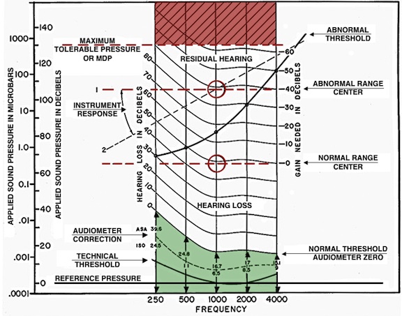
Figure 1. Otometric chart upon which all of the usually described measurement values of this post are shown in proper relation to each other. The chart was designed at a time when audiometers were calibrated to ASA Standards. For use with current Standards values (ANSI S3.6), all curved lines would be changed to conform to the dashed line shown under “audiometer correction.” This dotted line curve is plotted for audiometric ISO corrections, but is close to current pressures required for audiometric zero, and sufficiently similar for purposes here. The “abnormal range center” changes, depending on the “abnormal threshold.” It approximates the midpoint of the dynamic range at 1000 Hz. On the other hand, the “normal range center” is roughly fixed at about 65 dB SPL at 1000 Hz when measured under earphones, but 72 dB SPL when measured in a sound field. And, it is the latter that is most significant because both the normal ear, as well as an aided ear, operate in the sound field. As a result, otometry is based on sound field performance at most comfortable loudness.

As a specific example, at about 0.36 microbar, a sound pressure at 65 re 0.0002 microbar (65 dB re 0.0002 dynes/cm² or 65 dB re 20 µPa) at 1000 Hz, is roughly considered the normal range center and also the approximate pressure at which the 1000-Hz components of speech are normally received.

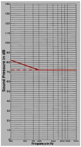
Figure 2. Shown is the free field (FF), or sound field Most Comfortable Loudness Pressure (MCPL) for normal listeners (flat line at 72 dB SPL). However, because of upward spread of masking, a preponderance of low-frequency environmental noise, and relatively lesser importance of low frequencies below 750 Hz for word recognition, low-frequency adjusted MCPLs are rolled off in the low frequencies to illustrate the unaided norm, and the aided expectation

 

The curved lines represent equal loudness contours. This means that for a normal listener’s most comfortable loudness (MCL) at 1000 Hz, the sound pressure to reach that level would be about 65 dB SPL. At 500 Hz, the sound pressure to reach MCL would be about 83 dB SPL (follow the curved line). The actual SPL varies to produce equal loudness, depending on the frequency.

Normal Range Center – The “normal range center” of most comfortable loudness pressures is roughly fixed at about 65 dB SPL at 1000 Hz when measured under earphones, but 72 dB SPL when measured in a sound field (Figure 2). The latter value is most significant because both the normal ear, as well as an aided ear, operate in the sound field. It is because of this that otometry is based on sound field performance at most comfortable loudness. Figure 2 also represents the uncluttered graph (otogram) used for otometric testing. The chart shows also a correction for the MCLP at the low frequencies. The values were rolled off 3-dB/octave for each 10-dB of in-use gain below 1000 Hz. These adjustments were made for the following reasons: (1) upward spread of masking, (2) a preponderance of low-frequency environmental noise, and (3) relatively lesser importance of low frequencies below 750 Hz for speech discrimination. The solid red line serves also as the amplified listening objective.

Otometric Principles for the Hearing Aid as a Prosthetic Device

With this background in mind, and with the intention of providing a scientifically-justified hearing aid prescription, the salient otometric principles were as follows:

1. The hearing aid should be concerned with sound pressure sensing abilities that remain, not on those that have been lost, as measured audiometrically as Hearing Loss or Hearing Level (HL). In other words, a hearing aid applies sound pressure to hearing that remains (suprathreshold information), not to that which is lost (threshold information)! Therefore, residual hearing range should be considered in absolute (sound pressure in SPL) rather than relative (Hearing Loss) decibels. This difference is illustrated in Figure 3.

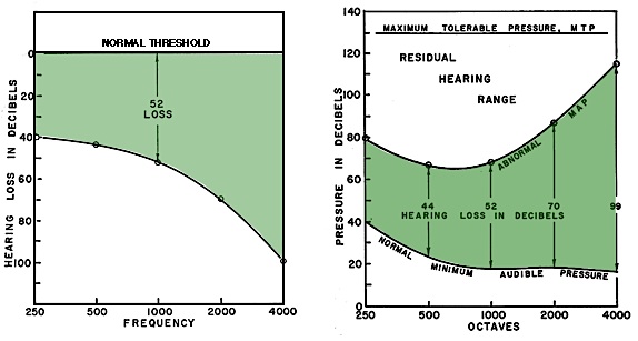
Figure 3. The audiogram (left) and hearing aid fittings based on it, calculate desired amplification from the level of the hearing loss threshold (a relative value). Otometry (right) bases amplification on sound pressure MCL (most comfortable loudness), an absolute value. This value, when measured, lies about half way between the recorded abnormal MAP (minimal audible pressure) and the MTP (maximum tolerable pressure). The comparisons are: normal threshold (Hearing Loss) compared to normal MAP, and hearing loss in relative dB compared to abnormal MAP in absolute sound pressure.

Most hearing aid fitting formulae are based on applying correction values to audiometric thresholds, levels at which even normal listening does not take place. Because of this, otometry sought to identify the most comfortable listening sound pressure level (MCLP) within the residual hearing range. It is this level at which individuals normally listen. Otometry then applied amplified hearing aid sound pressures to that level (Figure 4). This comfort range is only about 6 dB for normal hearing, and narrows with increasing hearing loss.

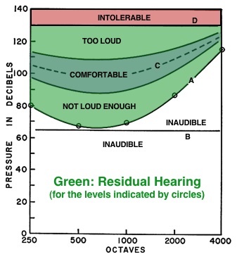
Figure 4. Otometric chart showing a residual hearing range having threshold pressures A, all of which are above the normally received level of line B. Pressures must be raised artificially with a hearing aid to line C to be most comfortable. Solid lines to either side of dashed line C define a latitude of comfortable loudness pressures.

2. Otometry predicts what is required to provide maximum utility of residual hearing and do not indicate how much, if any, intelligibility would result. The rationale for this is that from a hearing aid view, it makes no difference whether subnormal hearing is neurological or mechanical in nature.

3. Residual hearing and hearing aid properties are prescribed in terms of sound pressures required and sound pressures delivered. If the only measurements consist of conventional pure-tone threshold “Hearing Loss” values, these would have to be converted into corresponding minimum audible sound pressures for otometric purposes. But, even if this is done, minimum audible sound pressures (MAPs) are NOT part of the fitting prescription. They merely show the lower limit of the residual hearing range, which can be useful, along with the maximum tolerable pressures, to define the dynamic range from which a comfortable loudness pressure can be interpolated if/when the most comfortable listening pressures are not measured directly. Therefore, audiograms are not suitable for prescription purposes, and otometric charts (otograms) are used for evaluating residual hearing. In otometry, otograms and the hearing aid charts were designed with the same grids so that the measured hearing aid response could be superimposed on the residual hearing range to visualize how closely the hearing instrument comes to providing appropriate pressures to meet the comfortable loudness recommendation (Figure 5). The red line represents the measured hearing aid response compared to the comfortable listening level (blue area). In this example, the fitted hearing instrument provides comfortable listening in just two restricted regions, C and D. Adjustments would be required to provide as much of the measured hearing aid response (in sound pressure), to fall within the blue shaded area, as possible.

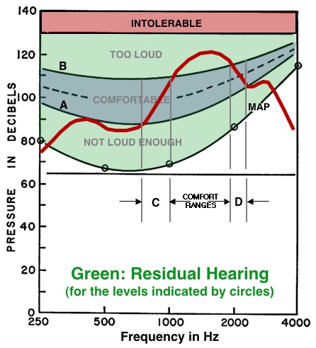
Figure 5. Otometric chart showing how the relative deliverable pressures (RDP) of a hearing aid (red line) can be superimposed upon the chart of an individual hearing range. The response of the hearing aid in this example shows that it can provide comfortable listening pressures in only two restricted regions, C and D, instead of distributing the pressures within the comfortable range between A and B. The comfortable level is for illustrative purposes only and does not reflect the most comfortable level pressures for a given individual.

4. Hearing aids/instruments are made to deliver sound pressure. As such, otometric measurement instruments must be more accurate than audiometric instruments if the possibilities of prescription are to be fully realized. In audiometry, thresholds are determined in 5-dB increments, meaning that at any frequency the result could be off by 10 dB because of ±5-dB variability. Pure tones are not acceptable stimuli to make the necessary loudness judgments because of fatigue when louder judgments are to be made, standing waves, etc., resulting in accuracy limitations.

Signal Used – A damped wavetrain (DWT) signal (Figure 6) was designed for use that is more like those produced by the parts of words of natural speech. This signal was selected for the following reasons:

• It was less prone to fatigue than a pure tone, and
• It allowed for a signal length that was no longer than necessary for recognition. Because signal duration varies with the number of cycles per second being delivered, providing the optimum number of cycles in the signal determines signal length. The number of cycles determined to be optimal was about 6 cycles per signal for the signal to be recognized. This suggested that for the same purposes, signals should be used that had the same number of cycles per signal, not the same time duration per signal as the frequency is changed.

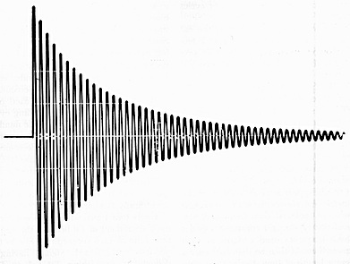
Figure 6. Oscillogram of the exponentially decaying (or damped) oscillatory signal. Each succeeding cycle reduces to 90% of the amplitude of the preceding cycle.

• Speech and other complex signals contain many individual frequency components, and therefore cannot supply information on a discrete or single frequency basis (needed for most comfortable pressures across the frequency range).
• A wavetrain signal has a repeatable number of cycles. Therefore, as a decaying signal, the decay rate is not specified in time, but in percent of amplitude retained in each succeeding cycle (Figures 6 ). A loss of 10% per cycle indicates that 90% remains, so that the decrement is then specified as being equal to 0.90. The signal decreases to about 1/2 amplitude in 6 cycles. The spectral distribution is constant throughout the signal presentation^[2].

5. Free-field (or sound-field) measurements are recommended because both the normal ear, as well as an aided ear, operate in the sound field.

6. Otometry was designed for a closed earmold coupler fitting. Substantial modifications would have to be made for other types of earmold coupling.

7. An adjustable volume control on the hearing aid is important for an otometric prescription fitting.

References

1. Victoreen JA. Hearing enhancement, Springfield: Charles C. Thomas; 1960.
2. Victoreen JA. The prescription of hearing aid instruments, Audecibel 1968;Spring:49–56, 58, 60–61.
3. Victoreen, JA. Hearing instruments and loudness, Audecibel 1972:190, 191–194, 196–198, 200–202.
4. Victoreen JA. Basic principles of otometry. Springfield: Charles C. Thomas; 1973.
5. Victoreen JA. Basic otometric principles, Audecibel 1973;Spring:63–70, 72–76, 78,79.